Demonstrating the existence of proportional error in mass spectrometry measurements.
mass-spectrometry
proportional-error
omics
metabolomics
Author
Robert M Flight
Published
April 9, 2021
Introduction
The other day, Kareem Carr asked for a statistics / data science opinion that results in the daggers being drawn on you (Carr, n.d.), and I replied (Flight, n.d.):
Every physical analytical measurement in -omics suffers from some proportional error. Either model it (neg binomial in RNA-seq for example), or transform your data appropriately (log-transform).
This includes DNA microarrays, RNA-seq, Mass Spec, and NMR (I need data to confirm)
I wanted to give some proof of what I’m talking about, because I don’t think enough people understand or care. For example, if you get mass-spec data from Metabolon, their Surveyor tool defaults to using non-log-transformed data. Trust me, you should log-transform the values.
Example Data
I have some direct-injection mass spec data on a polar fraction examining ECF derivatized amino-acids, with multiple “scans” from a Thermo Fisher Fusion Tribrid Mass Spectrometer. Each scan is the product of a small number of micro-scans. However, based on the spectrometer, and the lack of chromatography, it would not be unreasonable to expect that each scan is essentially a “replicate” of the other scans, so comparing one to any other is reasonable.
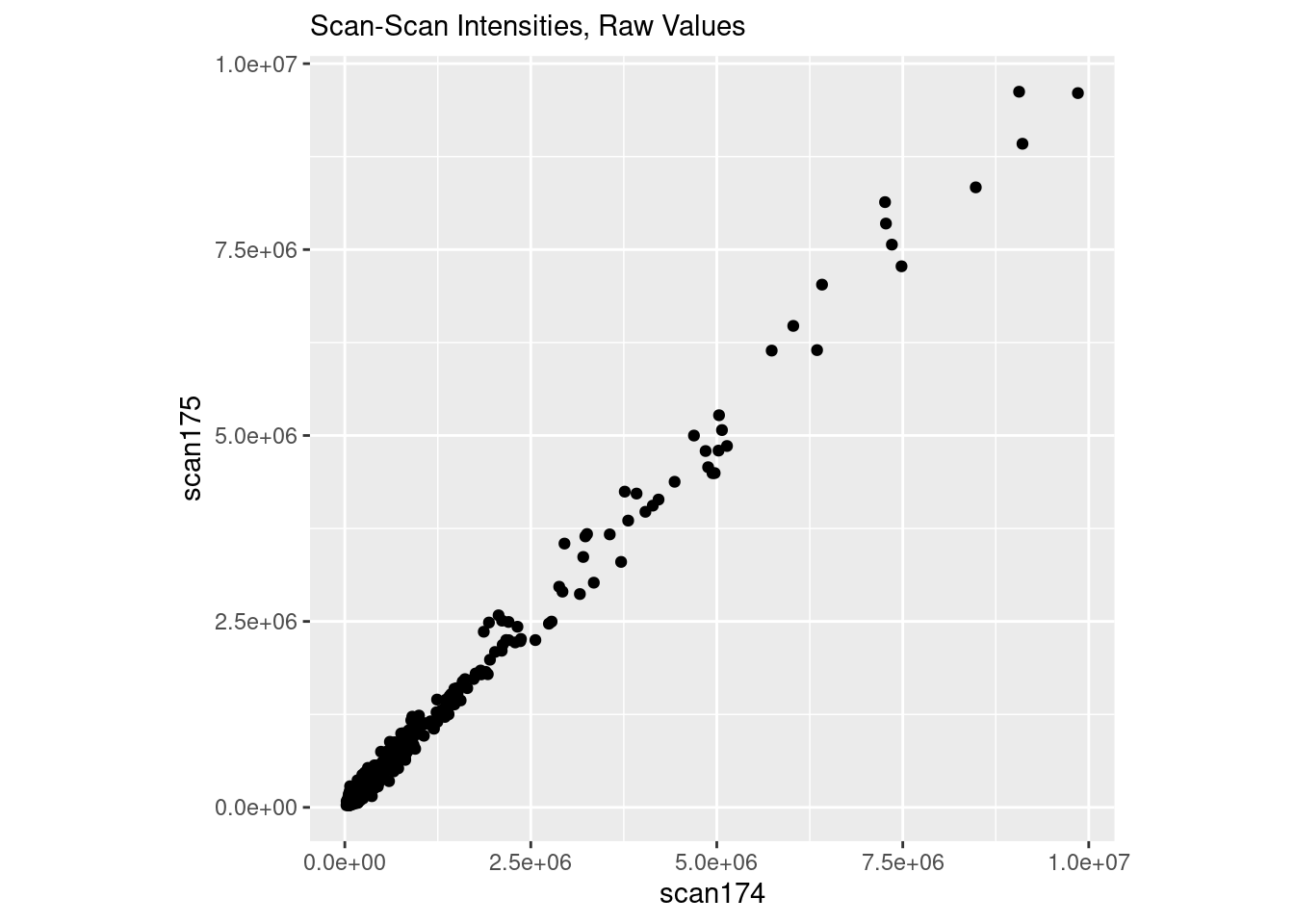
I’m going to load up the data, and plot two scans in “raw” space. The data are already log10 transformed, so we will “untransform” it back to “raw” first before plotting it.
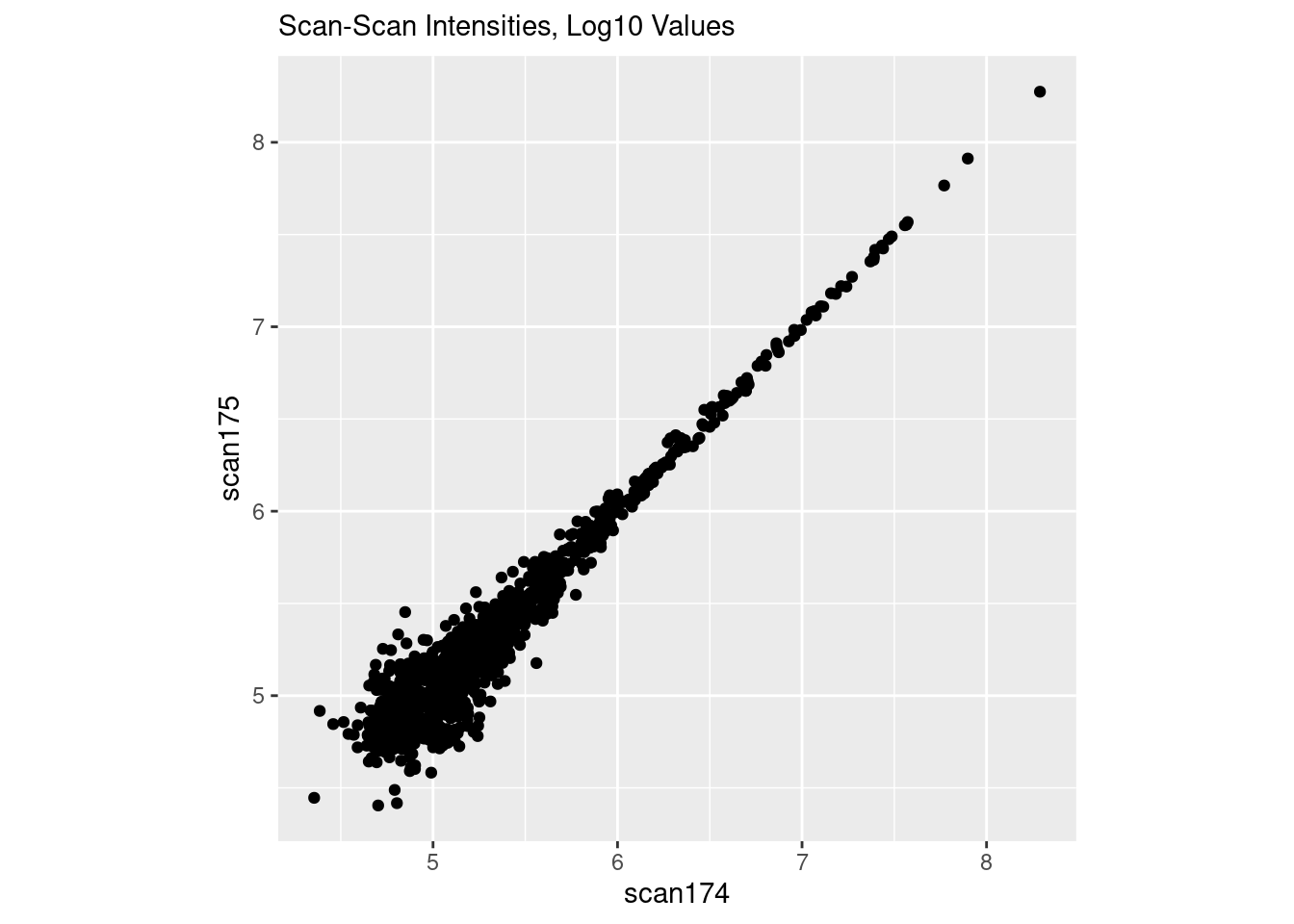
And now everything is coming to a point as the intensity increases.
If you’ve worked with microarray or RNASeq data, this is also commonly seen in those data.
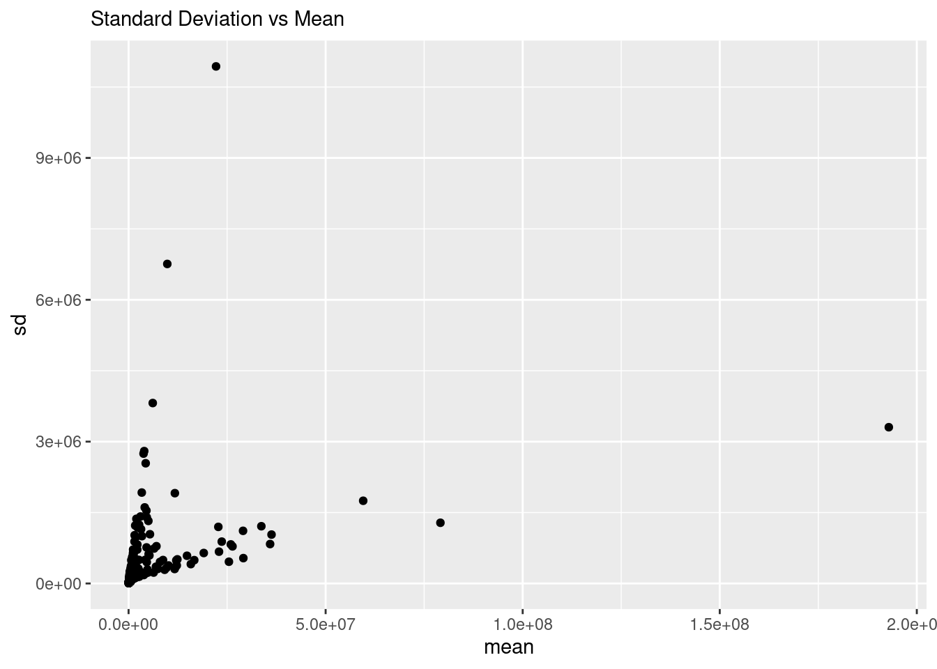
To show the presence of the proportional error more generally, we can calculate the mean and variance of each point across the scans, and plot those. To make sure we are getting “good” representations of the data, we will only use points that were present in at least 20 scans.
There you have it, the standard deviation is increasing with the mean, and doing so in two different ways, one increasing slowly, and one increasing quickly. Either of these are not good. Whether increasing slowly or quickly, the point is that the error / variance / standard deviation is somehow dependent on the mean, which most standard statistical methods do not handle well. This actually drove the whole development of using the negative-binomial distribution in RNASeq!
Why??
Why does this happen? Try this thought experiment:
I take 5 people in a room, and ask you to count how many people are in the room in 60 seconds and give me an answer.
I ask you to do this 20 times.
Your answer should be 5 each time, right?
Now I put 10 people in the room, and ask again how many are there. And ask multiple times.
Now 20 people in the same size room.
And then 30 people …
And then 40 people …
And so on.
If you think about it, given an constantly sized room, it will get harder and harder to count the people in it as their number increases, and with repeated counting, your estimates are likely to have more and more variance or a higher standard deviation as the number of people goes up. Thus the “error” is proportional or depends on the actual number of things you are estimating, much like the mass spec data above.
In DNA microarrays and RNA-seq, the technology was measuring photons. The higher the number of photons, the more difficult it is to be sure how many there are. And that gets translated to any downstream quantity based on the number of photons.
In Fourier-transform mass spectrometry, the instrument is still trying to quantify “how many” of each ion there is, and the more ions, the more difficult it is to quantify them. And we end up with proportional error.
I think in any technology that is trying to “count” how many of something there is within a finite space, these properties will manifest themselves. You just have to know how to look.
Solution
In the short term, transform your data using log’s. In the long term, I think we need more biostatisticians working with more mass-spectrometry and NMR data to determine what the error structure is for more instruments and analytical measurement types.